Env:
- MS VS 2015 Enterprise
- R Tools for VS (RTVS_2016-03-04.1.exe)
- MS R Open (MRO-3.2.4-win.exe)
- Math Library (RevoMath-3.2.4.exe)
dplyr package ( hadley/dplyr )
Key data structures
- data frames
- data tables
- SQLite
- PostgreSQL/Redshift
- MySQL/MariaDB
- Bigquery
- MonetDB
- data cubes with arrays (partial implementation)
> install.packages('dplyr')
Convert data to data frame
> data("mtcars")
> data('iris')
> mydata <- mtcars
> mynewdata <- tbl_df(mydata)
> myirisdata <- tbl_df(iris)
Convert data to data frame
> data("mtcars")
> data('iris')
> mydata <- mtcars
> mynewdata <- tbl_df(mydata)
> myirisdata <- tbl_df(iris)
> install.packages(c("nycflights13", "Lahman"))
> install.packages('RSQLite')
> install.packages('RPostgreSQL')
> library(dplyr) # for functions
> library(nycflights13) # for data nycflights13
> flights
Source: local data frame [336,776 x 16]
year month day dep_time dep_delay arr_time arr_delay carrier tailnum
(int) (int) (int) (int) (dbl) (int) (dbl) (chr) (chr)
1 2013 1 1 517 2 830 11 UA N14228
2 2013 1 1 533 4 850 20 UA N24211
3 2013 1 1 542 2 923 33 AA N619AA
4 2013 1 1 544 -1 1004 -18 B6 N804JB
5 2013 1 1 554 -6 812 -25 DL N668DN
6 2013 1 1 554 -4 740 12 UA N39463
7 2013 1 1 555 -5 913 19 B6 N516JB
8 2013 1 1 557 -3 709 -14 EV N829AS
9 2013 1 1 557 -3 838 -8 B6 N593JB
10 2013 1 1 558 -2 753 8 AA N3ALAA
.. ... ... ... ... ... ... ... ... ...
Variables not shown: flight (int), origin (chr), dest (chr), air_time (dbl),
distance (dbl), hour (dbl), minute (dbl)
# Caches data in local SQLite db
> flights_db1 <- tbl(nycflights13_sqlite(), "flights")
# Caches data in local postgres db
> flights_db2 <- tbl(nycflights13_postgres(), "flights")
# Caches data in remote postgres db
> nycflights13_postgres(host = 'local', port = '5432', dbname = 'nycflights13', user = 'nutt', password = 'nutt')
# Caches data in remote postgres db
> nycflights13_postgres(host = 'local', port = '5432', dbname = 'nycflights13', user = 'nutt', password = 'nutt')
Caching nycflights db in postgresql db nycflights13
Error in postgresqlNewConnection(drv, ...) :
RS-DBI driver: (could not connect nutt@local on dbname "nycflights13")
--- May be not found PostgreSQL in your env
--- Install and config program and replay steps again
Test PostgreSQL
> library('DBI')
> drv <- dbDriver("PostgreSQL")
> conn <- dbConnect(drv, host='local', port='5432', dbname='nycflights13', user='nutt', password='nutt')
> rs <- dbSendQuery(conn, "select * from pg_tablespace")
> fetch(rs, n = -1)
Single table verbs
- select(): focus on a subset of variables [ SELECT ]
> select(mynewdata, -c(cyl,mpg))
- filter(): focus on a subset of rows [ WHERE ]
> filter(myirisdata, Species %in% c('setosa', 'virginica'))
- mutate(): add new columns [ INTO ]
select(mpg, cyl)%>%
mutate(newvariable = mpg*cyl)
- summarise(): reduce each group to a smaller number of summary statistics [ GROUP BY ]
group_by(Species)%>%
summarise(Average = mean(Sepal.Length, na.rm = TRUE))
- arrange(): re-order the rows [ DESC | ASC ] i.e.
select(cyl, wt, gear)%>%
arrange(wt)
> system.time(carriers_df %>% summarise(delay = mean(arr_delay)))
> system.time(carriers_db1 %>% summarise(delay = mean(arr_delay)) %>% collect())
> system.time(carriers_db2 %>% summarise(delay = mean(arr_delay)) %>% collect())
Error in eval(expr, envir, enclos) : object 'carriers_db2' not found
> install.packages('plyr')
> system.time(plyr::ddply(flights, "carrier", plyr::summarise, delay = mean(arr_delay, na.rm = TRUE)))
Do() - applies any R function to each group of the data
> by_year <- lahman_df() %>%
+ tbl("Batting") %>%
+ group_by(yearID)
+ by_year %>%
+ do(mod = lm(R ~ AB, data = .))
> by_year %>%
+ do(mod = lm(R ~ AB, data = .)) %>%
+ object.size() %>%
22.7 Mb
> install.packages('biglm')
> by_year %>%
+ do(mod = biglm::biglm(R ~ AB, data = .)) %>%
+ object.size() %>%
+ print(unit = "MB")
0.8 Mb
* A lots of linear models consider use biglm instead of lm package. That 's good idea
Multiple table verbs - JOINS and SET
- inner_join(x, y): matching x + y
- left_join(x, y): all x + matching y
- semi_join(x, y): all x with match in y
- anti_join(x, y): all x without match in y
and
- intersect(x, y): all rows in both x and y
- union(x, y): rows in either x or y
- setdiff(x, y): rows in x, but not y
Recommend - load plyr first, then dplyr.
data table package ( Rdatatable/data.table )
> install.packages("data.table") # install it> library(data.table) # load it
> example(data.table) # run some examples
> ?data.table # read
> ?fread # read
> data("airquality")
> mydata <- airquality
> head(airquality, 6)
  Ozone Solar.R Wind Temp Month Day
1    41     190  7.4   67     5   1
2    36     118  8.0   72     5   2
3    12     149 12.6   74     5   3
4    18     313 11.5   62     5   4
5    NA      NA 14.3   56     5   5
6    28      NA 14.9   66     5   6
> data(iris)
> myiris <- iris
> library(data.table)
data.table 1.9.6  For help type ?data.table or https://github.com/Rdatatable/data.table/wiki
The fastest way to learn (by data.table authors): https://www.datacamp.com/courses/data-analysis-the-data-table-way

Attaching package: ‘data.table’

The following objects are masked from ‘package:dplyr’:

    between, last

Warning message:
package ‘data.table’ was built under R version 3.2.5
> mydata <- data.table(mydata)
> myiris <- data.table(myiris)
> mydata[2:4,]
> myiris[Species == 'setosa']
> myiris[Species %in% c('setosa', 'virginica')]
> mydata[,Temp]
> mydata[,.(Temp,Month)]
> mydata[,sum(Ozone, na.rm = TRUE)]
> mydata[,.(sum(Ozone, na.rm = TRUE), sd(Ozone, na.rm = TRUE))]
> myiris[,{print(Sepal.Length)
> myiris[, {
+     print(Sepal.Length)
+     plot(Sepal.Width)
+     NULL
+ } ]

ggplot2 Package ( hadley/ggplot2 )
ggplot2 is a plotting system for R, based on the grammar of graphics, which tries to take the good parts of base and lattice graphics and none of the bad parts. It takes care of many of the fiddly details that make plotting a hassle (like drawing legends) as well as providing a powerful model of graphics that makes it easy to produce complex multi-layered graphics.> library(ggplot2)
> library(gridExtra)
> bp <- ggplot(df, aes(x = dose, y = len, color = dose)) + geom_boxplot() + theme(legend.position = 'none')
> bp
 |
| Default boxplot |
i.e. without gridline
> bp + theme(panel.grid.major.y = element_blank(), panel.grid.minor.y = element_blank())
 |
| Boxplot without gridline |
What 's boxplot ?
 |
| Simple boxplot |
> sp <- ggplot(mpg, aes(x = cty, y = hwy, color = factor(cyl))) + geom_point(size = 2.5)
> sp
 |
| Scatterplot |
> bp <- ggplot(diamonds, aes(clarity, fill = cut)) + geom_bar() + theme(axis.text.x = element_text(angle = 70, vjust = 0.5))
> bp
 |
| Barplot |
Multi-graph on one page
> library(ggplot2)
Warning message:
package ‘ggplot2’ was built under R version 3.2.5
> library(gridExtra)
Warning message:
package ‘gridExtra’ was built under R version 3.2.5
> attach(mtcars)
The following object is masked from package:ggplot2:

    mpg

> p1 <- ggplot(ChickWeight, aes(x = Time, y = weight, colour = Diet, group = Chick)) +
+     geom_line() +
+     ggtitle("Growth curve for individual chicks")
+
> p1
> p2 <- ggplot(ChickWeight, aes(x = Time, y = weight, colour = Diet)) +
+     geom_point(alpha = .3) +
+     geom_smooth(alpha = .2, size = 1) +
+     ggtitle("Fitted growth curve per diet")
> p2
> p3 <- ggplot(subset(ChickWeight, Time == 21), aes(x = weight, colour = Diet)) +
+     geom_density() +
+     ggtitle("Final weight, by diet")
> p3
> p4 <- ggplot(subset(ChickWeight, Time == 21), aes(x = weight, fill = Diet)) +
+     geom_histogram(colour = "black", binwidth = 50) +
+     facet_grid(Diet ~ .) +
+     ggtitle("Final weight, by diet") +
+     theme(legend.position = "none")
> p4
> # Multiple plot function
+ #
+ # ggplot objects can be passed in ..., or to plotlist (as a list of ggplot objects)
+ # - cols:   Number of columns in layout
+ # - layout: A matrix specifying the layout. If present, 'cols' is ignored.
+ #
+ # If the layout is something like matrix(c(1,2,3,3), nrow=2, byrow=TRUE),
+ # then plot 1 will go in the upper left, 2 will go in the upper right, and
+ # 3 will go all the way across the bottom.
+ #
+ multiplot <- function(..., plotlist = NULL, file, cols = 1, layout = NULL) {
+     library(grid)
+
+     # Make a list from the ... arguments and plotlist
+     plots <- c(list(...), plotlist)
+
+     numPlots = length(plots)
+
+     # If layout is NULL, then use 'cols' to determine layout
+     if (is.null(layout)) {
+         # Make the panel
+         # ncol: Number of columns of plots
+         # nrow: Number of rows needed, calculated from # of cols
+         layout <- matrix(seq(1, cols * ceiling(numPlots / cols)),
+                     ncol = cols, nrow = ceiling(numPlots / cols))
+     }
+
+     if (numPlots == 1) {
+         print(plots[[1]])
+
+     } else {
+         # Set up the page
+         grid.newpage()
+         pushViewport(viewport(layout = grid.layout(nrow(layout), ncol(layout))))
+
+         # Make each plot, in the correct location
+         for (i in 1:numPlots) {
+             # Get the i,j matrix positions of the regions that contain this subplot
+             matchidx <- as.data.frame(which(layout == i, arr.ind = TRUE))
+
+             print(plots[[i]], vp = viewport(layout.pos.row = matchidx$row,
+                                       layout.pos.col = matchidx$col))
+         }
+     }
+ }
> library(grid)
> multiplot(p1, p2, p3, p4, cols = 2)
 |
| Multiplot |
reshape2 package ( hadley/reshape )
To makes easy to transform data between wide and long formats i.e.Wide format:
# ozone wind temp
# 1 23.62 11.623 65.55
# 2 29.44 10.267 79.10
# 3 59.12 8.942 83.90
# 4 59.96 8.794 83.97
Long format:
# variable value
# 1 ozone 23.615
# 2 ozone 29.444
# 3 ozone 59.115
# 4 ozone 59.962
# 5 wind 11.623
# 6 wind 10.267
# 7 wind 8.942
# 8 wind 8.794
# 9 temp 65.548
# 10 temp 79.100
# 11 temp 83.903
# 12 temp 83.968
Wide- to long-format data: the melt function
> aql <- melt(airquality)
No id variables; using all as measure variables
> aql <- melt(airquality, id.vars = c("month", "day"))
> head(aql)
  month day variable value
1     5   1    ozone    41
2     5   2    ozone    36
3     5   3    ozone    12
4     5   4    ozone    18
5     5   5    ozone    NA
6     5   6    ozone    28
> aql <- melt(airquality, id.vars = c("month", "day"),
+   variable.name = "climate_variable",
+   value.name = "climate_value")
> head(aql)
  month day climate_variable climate_value
1     5   1            ozone            41
2     5   2            ozone            36
3     5   3            ozone            12
4     5   4            ozone            18
5     5   5            ozone            NA
6     5   6            ozone            28
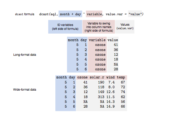
Long- to wide-format data: the cast functions
> aql <- melt(airquality, id.vars = c("month", "day"))
> aqw <- dcast(aql, month + day ~ variable)
> head(aqw)
  month day ozone solar.r wind temp
1     5   1    41     190  7.4   67
2     5   2    36     118  8.0   72
3     5   3    12     149 12.6   74
4     5   4    18     313 11.5   62
5     5   5    NA      NA 14.3   56
6     5   6    28      NA 14.9   66
 |
| http://seananderson.ca/2013/10/19/reshape.html |
 |
| http://www.analyticsvidhya.com/blog/2015/12/faster-data-manipulation-7-packages/ |
readr package ( hadley/readr )
Is slower than fread(), currently ~1.2-2x slower. If you want absolutely the best performance, use data.table::fread()
tidyr package ( )
- gather() – it ‘gathers’ multiple columns. Then, it converts them into key:value pairs. This function will transform wide from of data to long form. You can use it as in alternative to ‘melt’ in reshape package.
- spread() – It does reverse of gather. It takes a key:value pair and converts it into separate columns.
- separate() – It splits a column into multiple columns.
- unite() – It does reverse of separate. It unites multiple columns into single column
Gather()
> install.packages("tidyr")
Installing package into ‘E:/OneDrive/Rpackages’
(as ‘lib’ is unspecified)
trying URL 'https://cloud.r-project.org/bin/windows/contrib/3.2/tidyr_0.4.1.zip'
Content type 'application/zip' length 618746 bytes (604 KB)
downloaded 604 KB

package ‘tidyr’ successfully unpacked and MD5 sums checked

The downloaded binary packages are in
 C:\Users\nutt\AppData\Local\Temp\Rtmp2rxCdr\downloaded_packages
> library(tidyr)
Warning message:
package ‘tidyr’ was built under R version 3.2.5
> library(dplyr)

Attaching package: ‘dplyr’

The following objects are masked from ‘package:stats’:

    filter, lag

The following objects are masked from ‘package:base’:

    intersect, setdiff, setequal, union

Warning message:
package ‘dplyr’ was built under R version 3.2.5
> names <- c('A', 'B', 'C', 'D', 'E', 'A', 'B')
> weight <- c(55, 49, 76, 71, 65, 44, 34)
> age <- c(21, 20, 25, 29, 33, 32, 38)
> Class <- c('Maths', 'Science', 'Social', 'Physics', 'Biology', 'Economics', 'Accounts')
> tdata <- data.frame(names, age, weight, Class)
> head(tdata)
  names age weight     Class
1     A  21     55     Maths
2     B  20     49   Science
3     C  25     76    Social
4     D  29     71   Physics
5     E  33     65   Biology
6     A  32     44 Economics
> long_t <- tdata %>% gather(Key, Value, weight:Class)
Warning message:
attributes are not identical across measure variables; they will be dropped
> head(long_t)
  names age    Key Value
1     A  21 weight    55
2     B  20 weight    49
3     C  25 weight    76
4     D  29 weight    71
5     E  33 weight    65
6     A  32 weight    44
>
Separate()
> Humidity <- c(37.79, 42.34, 52.16, 44.57, 43.83, 44.59)
> Rain <- c(0.971360441, 1.10969716, 1.064475853, 0.953183435, 0.98878849, 0.939676146)
> Time <- c("27/01/2015 15:44", "23/02/2015 23:24", "31/03/2015 19:15", "20/01/2015 20:52", "23/02/2015 07:46", "31/01/2015 01:55")
> d_set <- data.frame(Humidity, Rain, Time)
> separate_d <- d_set %>% separate(Time, c('Date', 'Month', 'Year'))
Warning message:
Too many values at 6 locations: 1, 2, 3, 4, 5, 6
> separate_d
  Humidity      Rain Date Month Year
1    37.79 0.9713604   27    01 2015
2    42.34 1.1096972   23    02 2015
3    52.16 1.0644759   31    03 2015
4    44.57 0.9531834   20    01 2015
5    43.83 0.9887885   23    02 2015
6    44.59 0.9396761   31    01 2015
Unite()
> unite_d <- separate_d %>% unite(Time, c(Date, Month, Year), sep = "/")
> unite_d
  Humidity      Rain       Time
1    37.79 0.9713604 27/01/2015
2    42.34 1.1096972 23/02/2015
3    52.16 1.0644759 31/03/2015
4    44.57 0.9531834 20/01/2015
5    43.83 0.9887885 23/02/2015
6    44.59 0.9396761 31/01/2015
Spread()
> wide_t <- long_t %>% spread(Key, Value)
> wide_t
  names age     Class weight
1     A  21     Maths     55
2     A  32 Economics     44
3     B  20   Science     49
4     B  38  Accounts     34
5     C  25    Social     76
6     D  29   Physics     71
7     E  33   Biology     65
No comments:
Post a Comment